♾️ Infinite Widths Part I: Neural Networks as Gaussian Processes

This is the first post of a short series on the infinite-width limits of deep neural networks (DNNs). We start by reviewing the correspondence between neural networks and Gaussian Processes (GPs).

Visualising the NNGP correspondence. Empirical distribution of the 2D output of a 3-layer ReLU network over many random initialisations while increasing the width by a factor of 2.

TL;DR

Neural Network as Gaussian Process (NNGP): At initialisation, the output distribution of a neural network (ensemble) converges to a multivariate Gaussian as its width goes to infinity.

In other words, in the infinite-width limit, predicting with a random neural network is the same as sampling from a specific GP.

Brief history

The result was first proved by Neal (1994) for one-hidden-layer neural networks and more recently extended to deeper networks [2][3] including convolutional [4][5] and transformer [6] architectures. In fact, it turns out that any composition of matrix multiplications and element-wise functions can be shown to admit a GP in the infinite-width limit [7].

What is a Gaussian Process (GP)?

A GP is a Gaussian distribution over a function. More precisely, the function output for a set of inputs \(\{f(x_i, \dots, f(x_n)\}\) is jointly distributed as a multivariate Gaussian with mean \(\boldsymbol{\mu}\) and covariance or kernel \(K\), denoted as \(f \sim \mathcal{GP}(\boldsymbol{\mu}, K)\). See this Distill post for a beautiful explanation of GPs.

Intuition behind the NNGP result

There are different ways to prove the NNGP correspondence, to different levels of rigour and generality. Here, we will focus on the original derivation of Neal (1994) for one-hidden-layer network of width \(N_\ell\), before giving some intuition on the extension to deeper networks. Consider the \(i\)th neuron in the output layer

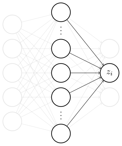
where we denote the hidden layer post-activation as \(h_j(x) = \phi(b_i^{(1)} + \sum_{k}^{N_0} W_{jk}^{(1)} x_k)\) with activation function \(\phi\). All the weights and biases are initialised i.i.d. as \(b_i^{(l)} \sim \mathcal{N}(0, \sigma_b^2)\) and \(W_{ij}^{(l)} \sim \mathcal{N}(0, \sigma_w^2/N_\ell)\). Note that, similar to standard (e.g. LeCun, Kaiming) initialisations, we rescale the variance of the weights by the width \(N_\ell\) to avoid divergence when applying the central limit theorem (CLT) to the pre-activations at the first feedforward pass. We would like to understand the prior over functions induced by this prior over parameters.

The NNGP result follows from two key observations:

1. Even though they receive the same input \(x\), all the hidden neurons \(h_j(x)\) are uncorrelated with each other because of independent parameters, and the nonlinearity is applied separately to each neuron. (Note that this breaks down for deeper layers at finite width.)
2. Any output neuron \(z_i(x)\) is a sum of iid random variables. Therefore, as \(N \rightarrow \infty\), CLT tells us that \(z_i(x)\) will converge to a Gaussian distribution. For multiple inputs, this will be a joint multivariate Gaussian, i.e. a GP. Note that the output neurons also become independent despite using the same “features” or inputs.

What are the mean and covariance of this GP? The mean is easy: since all the parameters are centered at initialisation, the mean of the GP is also zero.

where \(\theta\) represents the set of all parameters. The covariance is a little bit more involved

where we used the fact that the weights are independent for different inputs. We see that, in addition to the initialisation variances, the kernel depends on the activation function \(\phi\). For some nonlinearities we can compute the kernel analytically, while for others we can simply solve a 2D integral.

This is the key result first proved by Neal (1994). More recent works showed that this argument can be iterated through the layers by conditioning on the GP of the previous layer [2]

with initial condition \(K^0(x, x') = \sigma^2_b + \frac{\sigma^2_w}{N_0} x x'\). An alternative way of deriving this result is to notice that, even at finite width, the post-activation of any layer \(z_i^l(x)\) is a GP conditioned on the covariance of the previous layer and that this kernel becomes deterministic as the width grows to infinity.

Why does this matter?

This is one of the first results giving us a better insight into the highly dimensional functions computed by DNNs. Indeed, similar analyses had been previously carried out to characterise the “signal propagation” in random networks at initialisation [8][9][10]. Intuitively, if you have two inputs \(x\) and \(x'\), you don’t want their correlation to vanish or explode as they move through network, which would in turn lead to vanishing or exploding gradients, respectively.

In addition, since an infinite-width DNN is a GP, one can perform exact Bayesian inference including uncertainty estimates without ever instantiating or training a neural network. These NNGPs have been found to outperform simple finite SGD-trained fully connected networks [2]. For convolutional networks, however, the performance of NNGPs drops compared to their finite width counterparts, as useful inductive biases such as translation equivariance seem to be washed away in this limit [4].

In the next post of this series on the infinite-width limits of DNNs, we will look at what happens during training.

References

[1] R. M. Neal. Priors for infinite networks (tech. rep. no. crg-tr-94-1). University of Toronto, 1994

[2] Lee, J., Bahri, Y., Novak, R., Schoenholz, S. S., Pennington, J., & Sohl-Dickstein, J. (2017). Deep neural networks as gaussian processes. arXiv preprint arXiv:1711.00165.

[3] Matthews, A. G. D. G., Rowland, M., Hron, J., Turner, R. E., & Ghahramani, Z. (2018). Gaussian process behaviour in wide deep neural networks. arXiv preprint arXiv:1804.11271.

[4] Novak, R., Xiao, L., Lee, J., Bahri, Y., Yang, G., Hron, J., ... & Sohl-Dickstein, J. (2018). Bayesian deep convolutional networks with many channels are gaussian processes. arXiv preprint arXiv:1810.05148.

[5] Garriga-Alonso, A., Rasmussen, C. E., & Aitchison, L. (2018). Deep convolutional networks as shallow gaussian processes. arXiv preprint arXiv:1808.05587.

[6] Hron, J., Bahri, Y., Sohl-Dickstein, J., & Novak, R. (2020). Infinite attention: NNGP and NTK for deep attention networks. In International Conference on Machine Learning (pp. 4376-4386). PMLR.

[7] Yang, G. (2019). Wide feedforward or recurrent neural networks of any architecture are gaussian processes. Advances in Neural Information Processing Systems, 32.

[8] Poole, B., Lahiri, S., Raghu, M., Sohl-Dickstein, J., & Ganguli, S. (2016). Exponential expressivity in deep neural networks through transient chaos. Advances in neural information processing systems, 29.

[9] Schoenholz, S. S., Gilmer, J., Ganguli, S., & Sohl-Dickstein, J. (2016). Deep information propagation. arXiv preprint arXiv:1611.01232.

[10] Xiao, L., Bahri, Y., Sohl-Dickstein, J., Schoenholz, S., & Pennington, J. (2018). Dynamical isometry and a mean field theory of cnns: How to train 10,000-layer vanilla convolutional neural networks. In International Conference on Machine Learning (pp. 5393-5402). PMLR.